- Clasificación de un ráster
- Cálculo de Bandas
- Descripción de la calculadora de bandas
- Realizar un cálculo
- Opciones de salida
- Salvar y cargar expresiones
- Definición de regiones de interés
- Perfiles de imagen
- Árboles de decisión
- Funciones de Transformación Multiespectral
- Fusión de Imágenes
- Diagramas de dispersión
- Mosaicos
Clasificación de un ráster
Clasificación supervisada
Descripción funcionalidad
The main objectif of classifying an image according to previously established parameters is one of the most common goal of the remote sensing users. This tool allows to obtain classified maps derived from remote sensing data.
Thus the final goal is to produce a single band image, having same size and characteristiques of the original one, with the difference that single pixel value is a label identifying the category, among the selected ones, to which the pixel has been assigned during the classification procedure.
Clasificación supervisada de un ráster en gvSIG
gvSIG allows to perform a raster supervised classification by three different methods: maximum likelihood, minimum distance and parallelepiped.
To open the classification tool, you have to use the remote sensing toolbar by selecting “Raster process” from the left button and “Classification” from the right button.

The following window will be displayed
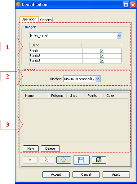
Operations Panel
In (1) choose the raster to classify. You can choose only an image already loaded in the view. For the selected image, chose also the bands you use to perform the classification process.
In (2) choose the method you use to perform the classification, you can select between: maximum likelihood, minimum distance and parallelepiped.
In (3) edit the classes on which the classification will be performed. By default, when you select the image to classify, a number of classes equal to the number of regions of interest (ROIs) linked to image are loaded.
You can modify (see document of ROIs editing) class number and composition, according to your need, without modifying the original ROIs.
Options Panel
To setup the parameters and the output options, activate the Option panel
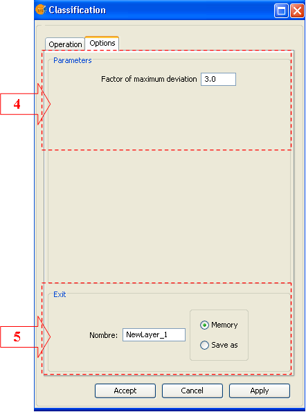
In (4) adjust the maximum standard deviation if the selected method is the parallelepiped one. In case of other methods, the panel will be empty.
In (5) setup the usual output parameters. Choose the output file name and path.
Cálculo de Bandas
Descripción de la calculadora de bandas
Band calculator allows you to perform mathematical operations between band values of the same image or from different images maintaining some spatial constraints (always on original values). The result of this operation is a one-band raster image.
To open the Calculator tool, you have to use the remote sensing toolbar by selecting “Raster process” from the left button and “Raster calculator” from the right button.
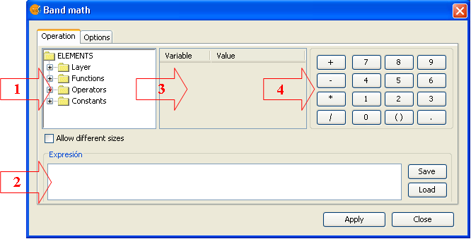
- the elements tree: allows to add different elements to the operation just browsing and double click over the selected element.
- expression frame: expression used for the operation
- table of variables: will contain the relation between variables and bands
- calculator keyboard: allow to insert numerical values as well as basic operators in the expression.
Realizar un cálculo
To perform a calculation among bands, you have to introduce an expression in the expression frame and link one band of the raster layers loaded in the TOC to one of the variables listed in the expression.
Write the expression in the expression frame. To do that, you can use all the elements of the calculator.
The decision tree contains the raster layer bands, functions, operators and constants that can be used to compose the expression. Make double click on the chosen element to introduce it in the expression (in the position where the cursor is located). For the bands, you will introduce a varaible that will be automatically associated to the band in the variables table.
Use the keyboard of the calculator to introduce numbers, operators, parenthesis and decimal separator in the expression.
In the variables table you can establish the association between the variables present in the expression and the bands of the raster layer. To link one band to one variable, or to change a link, select the table and double click over the desired band in the decision tree.
Check the box “Allow different dimensions” if you want that the bands having different dimensions, position or pixel size will be part of the calculation. This option involve the use of interpolation to obtain a result.
The result of a calculation is a one band raster layer, of type double, that contain the result of the expression for the pixels presents in ALL the input bands and the “no-data” value for the others.
Opciones de salida
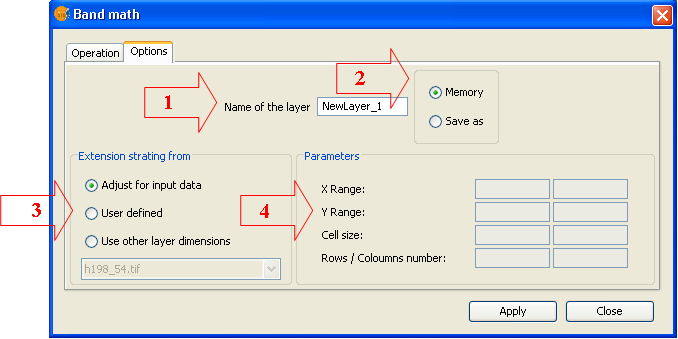
In this window you can select the options for the generation of the calculus result.
Name of the layer (1): Introduce the name of the raster layer that will be loaded in the window as calculus result.
Destination of the result (2): Select if you prefer to save the result as a file or to keep in memory. In the first case you will be asked for the path and the name of the file as the calculation will start. If you choose to keep in memory, you can save it later trough the option “Save as” by clicking with the right mouse button over the corresponding layer in the TOC.
Extension of the resulting raster (3). You can choose the extension and the cell size from the following possibilities:
1. Adjust to the input data: The extension of the resulting raster layer will be the union of the single band extensions presents in the calculation. The resulting cell size will be the smaller one amongst the bands presents in the calculation.
2. User defined: Use this option to introduce in the frame Parameters (4) maximum and minimum X and Y values and the output cell size.
3. Use other layer extension: The extension of the resulting layer will assume the ones of the selected raster layer.
Salvar y cargar expresiones
Click the button Save of the main control panel of the band calculator to save the expression shown in the Expression frame. A dialog window will appear to input the path and the name of the output file.
Click the button Load of the main control panel of the band calculator to an expression previously saved. The expression has to be saved as .exp
Definición de regiones de interés
Descripción de Herramienta edición Rois
This tool allows defining Regions of Interest (ROIs) over one raster layer. These regions or areas of interest can be used to derive statistics, classification processes, creation of masks or other applications.
To launch the ROIs edit tool for one layer you have to use the remote sensing toolbar by selecting “Raster layer” from the left button and “Area of interest” from the right button. You have to check that in the scrolling text window, the layer over which you want to draw the ROIs is selected.

The following window allows defining new ROIs linked to the selected layer.
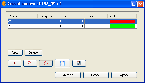
ROI definition step by step
Click over New. A new entry line corresponding to the new ROI will appear in the table. By default, new ROI does not contain any geometry.
Select the geometry you want for the new ROI by activating the corresponding control.
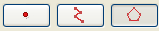
1- The first control allows to add a point to the selected ROI.
2- The second one a linear geometry.
3- The last one a polygon geometry.
Once selected the tool, draw the selected geometry aver the layer.
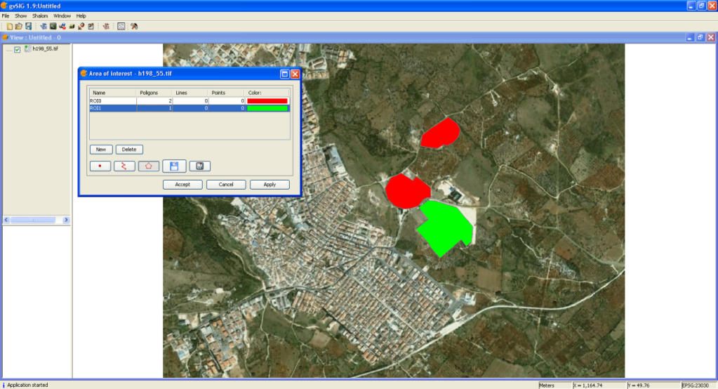
Add geometries over an already existing ROI
To add a new geometry to a ROI, select the corresponding ROI in the table.
Activate the corresponding control according to the geometry to add
Once drawn the geometry on the view, the ROI will be updated.
Delete a ROI
To delete a ROI select the corresponding line in the table.
Once selected the ROI, click on Delete.
Save a ROI as a shapefile
This option allows to export defined ROIs into a shapefile. The fields of this shapefile will be: (ROI name), R (R value in RGB), G (G value in RGB), and B (B value in RGB).
For each type of geometry linked to the selected ROIs, a Polygon, Polyline or Point file will be created that will manage the corresponding geometries of all the ROIs defined in the table.
Load ROIs from a shapefile
This option allows loading in the ROI tool regions defined by a shapefile. It is compulsory that the shapefile has the fields name, R, G, B. Additional fields can be present as well. Once loaded the ROI, it can be edited in the same way of any other ROI created with the ROI edit tool.
Perfiles de imagen
Descripción Herramienta de Perfiles
This tool allows visualising as a graphic the spectral profile of one point of the image (Z Profile) or the profile of a series of pixel belonging to a path drawn by the user.
To open the Profiles visualization tool, you have to use the remote sensing toolbar by selecting “Raster layer” from the left button and “Image profile” from the right button. You have to check that in the scrolling text window, the layer over which you want to visualize the profiles is selected.

The following window allows to define profiles over the layer.
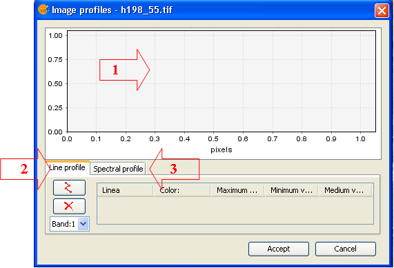
- Area over which you the graphic corresponding to the created profiles is drawn.
- Line profile. Panel to edit and visualize path profiles.
- Spectral profile. Panel to edit and visualize points spectral profiles.
Line profile
The panel to manage the line profiles disposes, in addition to the table, of the following controls

Add a new profile to the table. Once activated the control you draw the desired path over the view.

Delete the selected profile in the table by deleting the linked geometry and the graphic.

Select the band for which the profile will be created.
Spectral profile
The panel to manage point profiles has the following additional controls.

Add a new profile to the table. By control activation you choose the point on the image.
Delete the profile selected in the table by deleting the linked geometry and the graphic.
Árboles de decisión
Descripción funcionalidad de Árboles de decisión
Decision trees are used to represent and classify a list of conditions that can occur one after the other in order to obtain a classification of image pixel values.
To open the Decision tree tool, you have to use the remote sensing toolbar by selecting “Raster proces” from the left button and “Decision tree” from the right button.

Decision tree tool will appears as follow.
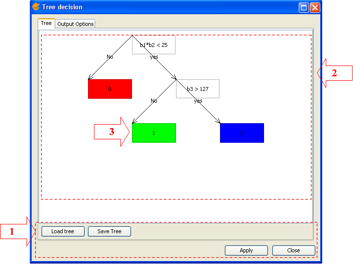
Description of the basic elements
- Menu.
From the Tree panel you can save or load a decision tree. By clicking on Close, you close the entire tool.
- Editing Decision tree panel.
On this panel you draw all the nodes that will affect the final tree configuration.
- Condition Nodes
To set up the tree, it is necessary to add and edit the decision nodes. Decision nodes are the ones appearing in colour in the panel. These nodes are linked to a Boolean expression whose evaluation, for each element of the selected variables, will lead to a result node or to a new evaluation node.
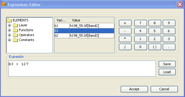
To add a new Condition Node it is necessary to click with the mouse right button (addChild) over a Result Node that you want to split. To assign the evaluation expression to the corresponding node, double click on the node and setup the condition by the expression editor that is shown in the following figure.
- Result Nodes or Leaf Nodes.
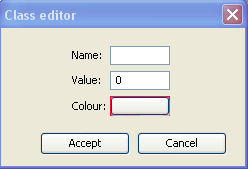
Each Decision Node has to two linked Leaf Nodes corresponding to positive or negative evaluation of the condition. These nodes appear coloured in the panel. They correspond to the assigned colour and value assigned in the result. These values can be modified from the window shown in the following figure and that can be activated by double click over the node.
Execution Options
Once edited the tree corresponding to the desired conditions, you can choose for a full execution or, on the contrary, for a partial execution starting from a given Condition Nodes. To perform the second option, it is necessary to activate the node contextual menu (right mouse button) and select ejecutar.
Output options
In the output options panel you can setup the parameters for the output raster.
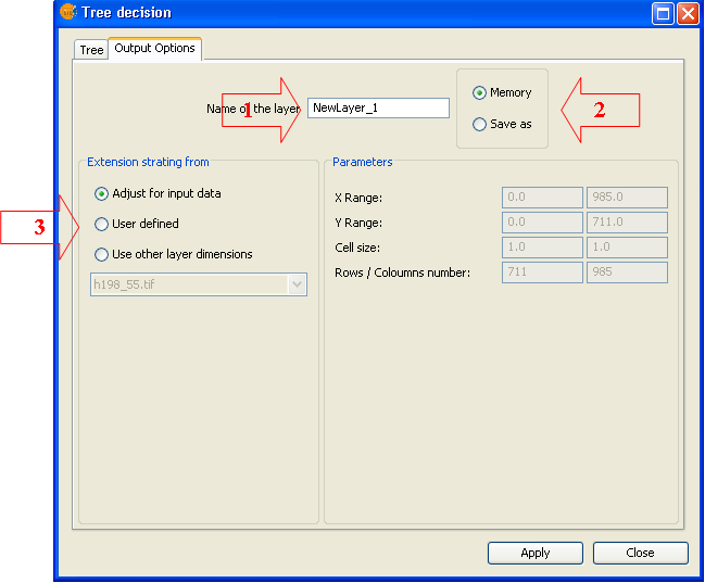
- File name
- Result file path: Select if you want to save the result as a file or to keep in Memory. In the first case you will be asked to specify the destination folder and the file name before launching the calculation. If you choose to keep in memory, you will be able to save it later by the option “Save as” by clicking with the right mouse button over the corresponding layer in the TOC.
- Extension of resulting raster. You can choose result dimension and pixel size as follow:
Adjust from input data: the raster dimension will consider pixel size of all the bands involved in the calculation. Smallest pixel size will be adopted as result.
User defined: Choose this option to input X and Y minimum and maximum values as well as resulting pixel size.
Use other layer dimensions: output raster dimension will assume the parameters of the selected raster layer
Funciones de Transformación Multiespectral
Descripción Funcionalidad de Componentes Principales
The principal components analysis is a multispectral transformation that whose goal is to avoid the use of redounding information in image bands. This technique allows transforming a list of bands into new variables called interlinked variables, absorbing most of data variability in an initial bands subset.
To open the Principal Components tool, you have to use the remote sensing toolbar by selecting “Raster process” from the left button and “Multispectral transformation” from the right button.

The dialog window will appears as follow.
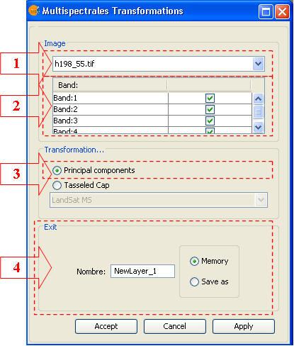
Step by step procedure to perform the transformation
- From the combo box, chose the image to which the transformation will be applied (1).
- Select the bands involved in the process in (2)
- Choose the Principal Components option. (3)
- Select output options. Select if you want to save the result as a file or to keep in Memory. In the first case you will be asked to specify the destination folder and the file name before launching the operation. If you choose to keep in memory, you will be able to save it later by the option “Save as” by clicking with the right mouse button over the corresponding layer in the TOC.
Start the process by Apply or Accept.
Later on, and during the analysis procedure, a dialog window similar to the one in the following figure will appear.
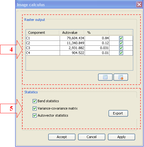
- Table fo components selection In this table you collect the information linked to every component calculated by the bands selected in the first window. The table include information of the corresponding autovalue and the percentage of variability absorbed by the component related to the total variability. The resulting image will be obtained according to the selected components
- Process statistics. The statistics generated in the previous procedure can be exported into a text file. To do this, every checkbox corresponding to the parameters must be selected, click on the option Export and select the path of the output file.
The image creation start by click on Apply or Accept. The result is a float image with as many bands as the selected components and it will automatically load in the view as the process finishes.
Descripción de Transformación Tasseled Cap
Tasseled Cap transformation aims to detect relevant spectral characteristics of developing vegetation surface, with the main goal to detect specific culture by the use of spectral ranges of multitemporal Landsat Images.
To open the Tasseled Cap tool, you have to use the remote sensing toolbar by selecting “Raster process” from the left button and “Multispectral transformation” from the right button.
The dialog window will appear as follow.
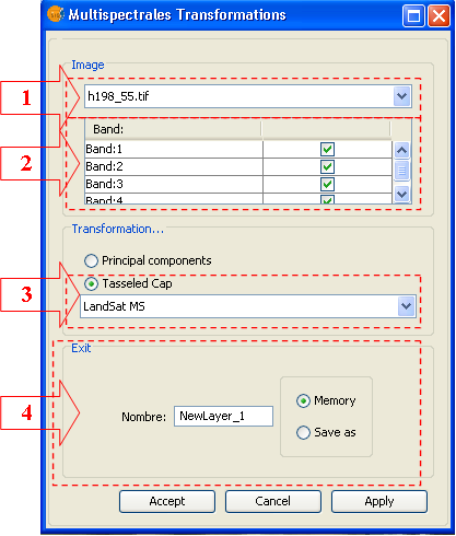
Step by step procedure to perform the transformation
- From the combo box, chose the image to which the transformation will be applied (1).
- Select the bands involved in the process in (2) The number of selected bands is strictly related to the transformation type that will be applied. Thus, for MS transformation 4 bands are needed while for TM and ETM, 6 bands. In the case of the band numbers does not fit transformation needs, the user will be informed.
- In the scroll menu choose the transformation type after having checked the Tasseled Cap checkbox. Transformation types are LandSat MS, LandSatTM and LandSat ETM+.
- Select output options. Select if you want to save the result as a file or to keep in Memory. In the first case you will be asked to specify the destination folder and the file name before launching the operation. If you choose to keep in memory, you will be able to save it later by the option “Save as” by clicking with the right mouse button over the corresponding layer in the TOC.
Start the process by Apply or Accept.
The result is a float image with as many bands as the selected components and it will automatically load in the view as the process finishes
Fusión de Imágenes
Descripción de funcionalidad de fusión de imágenes
The technique of combining images having different spectral or spatial resolution is called image fusion. The goal is to increment the resolution of images having a low spatial resolution using the corresponding panchromatic image. The result is a multispectral image having a resolution close to the panchromatic one.
To open the Image Fusion tool, you have to use the remote sensing toolbar by selecting “Raster process” from the left button and “Images fusion” from the right button.

The dialog window will appear as follow.
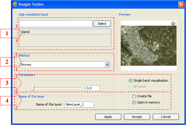
Description of the basic elements
- Panel to select the high resolution band
Using the button Select, chose the image or panchromatic band that will be used in the process.
- Panel to select the fusion method
- In this panel you select the fusion method. You can choose between :
- Brovey
- IHS
- Principal Components
- Wavelets
- Parameters Panel
In this panel you can setup the parameters of any single method listed in (2).
- Options panel
Output options include the possibility to name the output file as well as the usual management options. The result can be obtained just for the visualised bands as well as for all the raster bands.
Diagramas de dispersión
Descripcion funcionalidad de Diagramas de Dispersión
The goal of representing the dispersion is to graphically observe the correlation between couple of bands of an image. To visualize the dispersion diagram, use the Remote Sensing toolbar selecting “Raster layer” from the left button and “dispersion diagram” from the left button. Check that in the scrolling text window, the layer over which you want to perform the diagram is selected.

The dialog window will appear as follow.
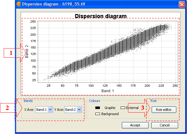
- Area where the graphic will be drawn. This graphic will change as the selected bands are changed. By default, the first graphic is created with band 1 and 2 of the image.
- Boxes of the selected bands.
- Option to show the graphic ROI editor.
Step by step to define new ROIs in the graphic
(1) Using the contextual menu

- Open the contextual menu over the diagram by right click.
- Choose New Class option
- Draw on the graphic the rectangular shape(s) delimiting ROI pixel values
(2) Using ROIs editor
- Click on ROIs Editor in the tool window. The editor will appear as follow

- By selecting "New" a new entry will be created in the table for managing the ROIs in the graphic. Then ROI name and colour can be modified. With the entry selected, draw rectangular(s) delimiting ROI pixel values in the represented bands.
Delete a ROI of the graphic
- Over the tool ROIs Editor select the entry corresponding to the ROI you want to delete.
- Click on "Delete"
Export a ROI of the graphic to a ROI in the layer
- Over the tool ROIs Editor select the entry corresponding to the ROI you want to export.
- Click on "Export"
- Once exported, the defined ROI will remain permanently linked to the image and will be managed as any other ROI created with the ROI editing. This new ROI will contain only point geometry
Mosaicos
Descripción funcionalidad de mosaicos
A mosaic is a match of two or more images edging or partially overlaying in order to create a single image of the area covered by the images. To elaborate a mosaic it is necessary that all the images are in the same projection.
To visualize the mosaic tool, use the Remote Sensing toolbar selecting “Raster process” from the left button and “Mosaics” from the left button.

The dialog window will appear as follow.
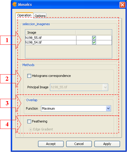
(1). Area of image selection. The images selected in this table are the ones that will compose the mosaic.
(2). As preliminary step to the composition of the mosaic, an Histogram Matching can be performed in order that all the images of the mosaic will be adjusted to the histogram of a reference image selected by the user in the combo box.
(3). Selection of the method to perform the mosaic. Available methods are
- Maximum: Maximum band value for all the overlaying pixels.
- Minimum: Minimum band value for all the overlaying pixels.
- Average: Arithmetical average value for all the overlaying pixels.
- Of the top image: Pixel values of the top image in the view are assumed
- Of the bottom image: Pixel values of the bottom image in the view are assumed
(4). Feathering Function. If the corresponding check box is activated, the mosaic is built by a procedure of edge degradation. This method allows that only two images are involved in the mosaic.
Output options
Output options are usual ones. Select if you want to save the result as a file or to keep in Memory. In the first case you will be asked to specify the destination folder and the file name before launching the operation. If you choose to keep in memory, you will be able to save it later by the option “Save as” by clicking with the right mouse button over the corresponding layer in the TOC.
-----------------------------------
- Se ha producido un error en el documento Descripcion funcionalidad de Diagramas de Dispersión , accediendo a la imagen dispersion_Rois.png, que probablemente no existe. No se han encontrado alternativas
